Let's explore MLflow, part 3: applying MLflow

Context

In my previous post, I established the scope and context for a demo data science project which would use MLflow to handle MLOps. How helpful - or inconvenient - would this be for tracking and comparing experiments over different machine learning pipelines? Is this an easy way to get, say, a leaderboard for model performacne that could be shared across a small team? Or, is this more trouble than it’s worth?

I’m happy to share that, barring a few notable challenges, MLflow was very convenient to work with in this demo. I’m quite pleased with how simple it is to set up a systematic workflow that takes advantage of MLflow’s tracking functionality. While I didn’t explore using MLflow for model deployment in depth, it’s also clear to me that the out-of-the-box functionality is quite powerful.

Here’s how I implemented the demo project. This will be a fairly long post, but it also contains pretty much everything one needs to replicate the demo.

The demo project

In order to run this experiment, I’ll need to define the following:

Assumptions

• Timestamps correspond to the start of the interval. It’s important to establish this convention before getting too far ahead - I’ve seen firsthand the chaos that can happen when handwaving this away!
• To make the problem more tractable, and more comparable to CAISO’s own day-ahead forecasts, let’s downsample the data to hourly resolution. In the previous post’s analysis, I examined the raw 5-minute data, but afterwards I realized that using a 1-hour resolution had several major advantages. As for downsides, this is a demo project so there isn’t much benefit to insisting on a 5-minute resolution anyway.
• Let’s also assume that in practice, input data would be available to the workflow (e.g. for inference and serving forecasts in production) immediately upon the end of an interval. For example, the actual system demand for 1/1/2025 1:00-1:59 PM would be published at 2:00 PM. This means that the workflow could then generate forecasts for 3:00 PM onward as early as possible after 2:00 PM. In reality, any external data sources will have some lag time due to their own processing activity, but this is not an unrealistic assumption for e.g. data sources which are hourly aggregates of 5-second live readings.
• Forecasts for day $d+1$ are to be performed on day $d$, between 2:00 PM and 3:00 PM local time. This also represents a realistic constraint for a day-ahead system demand forecast, which might only run once per day. In fact, this might be necessary if historical hourly system demand were only published by the system operator (here, CAISO) once daily. With the previous assumption, this means that only data through 1:59 PM of the same day are available at each inference time. The data processing workflow and model features will need to respect this in order to avoid leakage of future information.

Performance evaluation

My goal is to predict the day-ahead system demand at hourly resolution. That is, my desired model will forecast - each day sometime soon after 2:00 PM local time - the system demand at 3:00 PM, 4:00 PM, etc. through 2:00 PM of the next day.

Because I plan on generating one day-ahead forecast daily, without “course-correcting” by generating new forecasts inbetween, I care about the forecast error for all time steps in the forecast horizon. Assuming these are equally important, then, let’s define a model’s performance for one day as the average root mean squared error (RMSE) across all time steps in the horizon. Alternatively:

where $h$ is the horizon length (i.e. $h$-step-ahead forecast), $N$ is the number of samples (i.e. predictions made in the training/test set), and every sample $n$ has forecasts for all $h$ steps ahead in the maximum forecast length.

RMSE is a good choice for applications like this where large errors are disproportionately costly, e.g. where major mismatches in electricity supply and demand threaten power grid stability, since the square term in RMSE penalizes larger errors more than proportionally.

Training, validation, and test sets

The training dataset begins at 2018-01-01 00:00 and ends at 2024-12-31 23:00 local time (-08:00 UTC) . When performing hyperparameter optimization, I will use time series (rolling) cross validation to make sure that no “future” information leaks into the validation set.

I reserve the remainder of 2025 as a test set for final performance evaluation. This represents 2025-01-01 00:00 through 2025-05-02 23:00 local time.

Initial preprocessing

I implemented this project in a Jupyter notebook, and will include snippets from it below.

import getpass
import logging
import mlflow
from mlflow.models import infer_signature
import numpy as np
from numpy import nan
import pandas as pd
from pathlib import Path
import subprocess
from typing import List

logging.basicConfig(level=logging.DEBUG)

To get the data ready for the project’s “test harness”, I need to enforce the assumptions above.

• The timestamps in the raw files are timezone-naive datetimes supposed to be in local (America/Los_Angeles) time, so I will add a timezone-aware column "local_datetime" explicitly capturing this.
• I will also flag all observations corresponding to “inference times”, when a day-ahead forecast will be generated, in the column "inference". Eventually, the plan is to fit/predict at these times only. First I will need to build any features that might require lagged observations, though!
• In general, I prefer keeping datetime indices in UTC - this avoids unpleasant nonsense with daylight savings, cross-timezone comparisons, etc. So, I’ll convert the dataset index as well.
• There is one outlier with obvious data quality issues that I identified in the previous blog post, so I’ll drop that as well.
• Finally, I’ll perform the resampling from 5-minute to hourly frequency. System load for the hour is the average across the 5-minute intervals, which makes sense:
  • Each hour has 12 five-minute intervals, each with its own average MW (megawatts) power demand.
  • The total MWh (megawatt hours) energy demand for a five-minute interval is its MW power times its duration in hours (1/12).
  • The total MWh energy demand for the entire hour is the sum of the MWh energy demands for the 12 five-minute intervals that make it up.
  • Finally, the average MW power demand in the hour is the total MWh in that hour divided by the number of hours (one).

def load_prepare_csv(path_demand):
    df = pd.read_csv(path_demand, parse_dates=[0], index_col=0)

    # Flag inference timestamps based on local time
    df = df.tz_localize("America/Los_Angeles", ambiguous="infer")
    df["local_datetime"] = df.index
    df["inference"] = df.index.hour == 14

    # To UTC
    df = df.tz_convert("UTC")
    df = df.reindex(
        pd.date_range(
            df.index[0], df.index[-1], freq="5min", tz="UTC"
        )
    )

    # Drop known outlier from exploratory data analysis
    df.Load.at["2021-07-05 18:45+00:00"] = nan

    # Upsample to hourly
    df = df.resample(rule="1h").mean()
    # Correct for mean upsample operation
    df["local_datetime"] = df["local_datetime"].dt.floor("h", ambiguous="infer")
    df["local_datetime"] = df["local_datetime"].dt.tz_localize(None)  # See note
    return df

dir_data = Path(r"D:\Projects\Data\CAISO")
df = load_prepare_csv(dir_data.joinpath("demand_2018-2024.csv"))
df_holdout = load_prepare_csv(dir_data.joinpath("demand_2025_ytd.csv"))
df = pd.concat([df, df_holdout], axis=0)

Plug-and-play models and interfacing with the “test harness”

One of my goals with this project was to demonstrate how MLflow might make it easier for a team of data scientists to stick to a single, shared “test harness” that guarantees honest comparisons between different predictive models. For this test harness, just the inner models should be substitutable, and can be experimented with in parallel by different users. In order for this to work, though, the team would need every valid model to have a consistent interface that is compatible with the test harness.

Fortunately, MLflow makes it very easy to do this by providing exactly that!

In the official quickstart and tutorial guides that I explored in the first post in this series, the examples exclusively used scikit-learn classes. In fact, MLflow has built-in, streamlined functionality (“flavors”) for logging models that are implemented with many popular libraries:

• H2O (h2o)
• Keras (keras)
• PyTorch (pytorch)
• Scikit-learn (sklearn)
• Spark MLlib (spark)
• TensorFlow (tensorflow)
• ONNX (onnx)
• XGBoost (xgboost)
• LightGBM (lightgbm)
• CatBoost (catboost)
• Spacy (spaCy)
• Statsmodels (statsmodels)
• Prophet (prophet)
• Pmdarima (pmdarima)
• John Snow Labs (johnsnowlabs)
• Diviner (diviner)
• Transformers (transformers)
• SentenceTransformers (sentence_transformers)

However, arbitrary logic can easily be converted into a model that MLflow can work with by implementing it as a Python Function “flavor” model or even an R Function “flavor” model. For Python, the interface is provided by the mlflow.pyfunc.PythonModel class. As long as the custom model class inherits from this and implements its predict method appropriately (and, when necessary, its load_context method), then MLflow can use this!

The predict method for a custom model class needs to have a signature of either predict(self, model_input, params) or predict(self, context, model_input, params). What’s the difference between these? context is intended to represent artifacts that are used during prediction but are ideally loaded once, in advance (e.g. saved model weights). This contrasts with params which are key-value pairs that could change across inference runs (e.g. random seed). If a custom Python model class omits context from its predict implementation, then it is still valid, but assumes no special logic is needed to load artifacts for it to work.

from abc import abstractmethod

class AbstractDemandForecastModel(mlflow.pyfunc.PythonModel):
    def __init__(self, *args, **kwargs):
        pass

    @abstractmethod
    def fit(self, model_input, model_output):
        pass

    @abstractmethod
    def predict(self, model_input: np.ndarray, params=None) -> np.ndarray:
        pass

Note the explicit type hints on the predict method signature, which helps MLflow set up automated input validation!

So far, this is fairly straightforward. If all feature engineering and predictive modeling is in scikit-learn, then this isn’t even necessary - I could just use the MLflow model logging flavor for it and avoid a custom class! This is especially useful if, say, I wanted to perform feature engineering with scikit-learn estimators then pass the output to Tensorflow logic that was not itself wrapped in a class inheriting from sklearn.base.RegressorMixin.

However, I want to add some more complexity.

Suppose I want to decouple experimenting with feature engineering versus experimenting with model algorithms. Whenever a new feature engineering or model algorithm is developed, the team would want to test how it interacts with some or all of the other component’s variants. Allowing this could permit more efficient, parallel workstreams within the team so long as the test harness and MLflow support this.

In order to do this, the workflow should track “feature preprocessing models” and “regression models” separately. I’m sure there are many ways to accomplish this, but I identified two obvious approaches:

1. Implement feature preprocessing and regression separately, but chain them in a sklearn.pipeline.Pipeline and log that composite model. The composite model and its experiment runs would be tagged with one tag for the feature preprocessing class, and another tag for the regressor class. This is elegant and easy to implement, but unfortunately would not allow the team to deploy/rollback one stage independently of the other stage. In practice I’m not sure how important this is, but it seems like that would be valuable.
2. Implement feature preprocessing as its own mlflow.pyfunc.PythonModel child class, and log it separately. This is the more flexible approach, but requires deviating from scikit-learn’s transformer class conventions in one potentially confusing way: For MLflow to log and serve an arbitrary Python model, it must implement the predict method. Note that scikit-learn transformer classes don’t have this, and implement transform instead! Therefore, I need to break with the scikit-learn convention and implement predict according to mlflow.pyfunc.PythonModel’s method signature, but make it do what the transform method would do. In fact, I can implement transform too, and just have one call the other.

Let’s take the second approach:

class AbstractDemandFeatureProcessor(mlflow.pyfunc.PythonModel):
    def __init__(self, *args, **kwargs):
        pass

    @abstractmethod
    def fit(self, model_input, model_output=None):
        pass

    @abstractmethod
    def predict(self, model_input: pd.DataFrame, params=None) -> np.ndarray:
        """
        This should be equivalent to self.transform(X, y) since
        mlflow.pyfunc.PyFuncModel requires it to be logged correctly.
        """
        pass

    def transform(self, model_input, params=None):
        return self.predict(model_input, params=params)

The test harness

This logic is responsible for an “apples-to-apples” comparison across the experiment’s runs. Ideally, each data scientist on this project would use this without any modification to evaluate and persist candidate models.

It is absolutely critical that the test harness doesn’t allow any future information to contaminate model fitting and inference. At the same time, though, it would be much more efficient to perform certain operations like constructing time-lagged features on the entire dataset at once. The test harness has other responsibilities that include fitting both the feature preprocessing and regressor sub-models, evaluating them on the training (and optionally, test) datasets, applying tags to the experiment run, logging metrics, and persisting model artifacts for future recovery and eventual production deployment.

Here’s how I implemented it.

from sklearn.metrics import root_mean_squared_error

def make_multistep_horizon_target(y, steps=24):
  """
  Get the next 24 hours and make them a vector of size 24 to serve as
  the array-valued regression target.
  """
  return pd.concat([y.shift(i) for i in range(steps)], axis=1).values

def filter_inference_rows(A, B, C):
  """
  For arrays A, B, and C with the same row dimension, keep only
  the rows from A and B which have value True in C.
  """
  return A[C > 0], B[C > 0]

def filter_matched_nan_rows(A, B):
  """
  For two arrays with the same row dimension, find the rows
  which have any NaNs in either array and eliminate them from both.
  """
  keep_A = (~np.isnan(A)).all(axis=1)
  keep_B = (~np.isnan(B)).all(axis=1)
  keep_AB = keep_A & keep_B
  return A[keep_AB, ], B[keep_AB, ]

These helper functions come into play later.

• The first will efficiently construct the array-valued regression target, since I want to predict the next 24 hours in advance. Note that this is agnostic whether the regression model independently forecasts each time step, takes advantage of correlations between them, or even iteratively predicts them as with exponential smoothing or ARIMA models.
• The second will be used to filter both the predictor (A) and target (B) matrices to only those observations where the day-ahead forecast is to be generated (C). I don’t need to fit or backcast at times where a deployed forecasting system wouldn’t generate forecasts anyway! This will reflect the intended use case more closely and economize on resources, insofar as that matters here.
• The third will drop all records where either some predictor feature (A) or a target time horizon (B) has missing data. This is useful because at that point in the test harness, the predictor and target matrices will already be separate.

Here is the main function for the test harness:

def experiment_run(df, feature_preprocessor_class, model_class,
                   feature_preprocessor_params=dict(), model_params=dict(),
                   holdout_start_date: pd.Timestamp | None = None):
    # Validate param names are unique
    duplicate_param_names = set(feature_preprocessor_params.keys()).intersection(model_params)
    if len(duplicate_param_names) > 0:
        raise ValueError("Feature preprocessor params and model params should not share any names, "
                         f"but both had: {duplicate_param_names}")

    # Train/test split by date if provided
    if holdout_start_date:
        train_end_date = holdout_start_date - pd.Timedelta(seconds=1)
    else:
        train_end_date = df.index.max().isoformat()

    # Preprocess all the data and do feature engineering;
    #note that no operation here must use future observations!
    feature_preprocessor = feature_preprocessor_class(**feature_preprocessor_params)
    feature_preprocessor.fit(df.loc[:train_end_date])  # Calibrate on training data only...
    X = feature_preprocessor.predict(df)               # ...but prepare entire dataset in one pass
    Y = make_multistep_horizon_target(df["Load"])

    # Filter to training set
    X_train = X[df.index <= train_end_date]
    Y_train = Y[df.index <= train_end_date]

    # Only consider records where inference would be performed
    X_train, Y_train = filter_inference_rows(X_train, Y_train, df.loc[:train_end_date, "inference"])

    # Only consider complete records
    X_train, Y_train = filter_matched_nan_rows(X_train, Y_train)

    # Fit the model (including any hyperparameter optimization with time series cross-validation)
    model = model_class(**model_params)
    model.fit(X_train, Y_train)

    # Training data predictions
    Yh_train = model.predict(X_train)
    rmse_train = root_mean_squared_error(Y_train, Yh_train, multioutput="uniform_average")

    if holdout_start_date:
        # Evaluate on holdout test set
        # Filter to training set
        X_test = X[df.index > train_end_date]
        Y_test = Y[df.index > train_end_date]

        # Only consider records where inference would be performed
        X_test, Y_test = filter_inference_rows(X_test,
                                               Y_test,
                                               df.loc[df.index > train_end_date, "inference"])

        # Only consider complete records
        X_test, Y_test = filter_matched_nan_rows(X_test, Y_test)

        # Fit the model (including hyperparameter optimization with time series cross-validation)
        model = model_class(**model_params)
        model.fit(X_test, Y_test)

        # Holdout (test) data predictions
        Yh_test = model.predict(X_test)
        rmse_test = root_mean_squared_error(Y_test, Yh_test, multioutput="uniform_average")

    # Set our tracking server uri for logging
    mlflow.set_tracking_uri(uri="http://127.0.0.1:8080")

    # Select the MLflow Experiment, else create if does not exist yet
    mlflow.set_experiment("CAISO day-ahead system demand forecast")

    # Start an MLflow run
    with mlflow.start_run():

        # Log the dataset
        dataset_training = mlflow.data.from_pandas(df.loc[:train_end_date],
                                                   name="CAISO System Load", targets="Load")
        mlflow.log_input(dataset_training, context="training")
        if holdout_start_date:
            dataset_testing = mlflow.data.from_pandas(df.loc[holdout_start_date:],
                                                      name="CAISO System Load", targets="Load")
            mlflow.log_input(dataset_testing, context="testing")

        # Log the hyperparameters
        mlflow.log_params(feature_preprocessor_params | model_params)

        # Log the loss metric
        mlflow.log_metric("rmse_train", rmse_train)
        if holdout_start_date:
            mlflow.log_metric("rmse_test", rmse_test)

        # Tag the class names of the used objects
        mlflow.set_tag("feature_preprocessor_class", feature_preprocessor_class.__name__)
        mlflow.set_tag("model_class", model_class.__name__)

        # Tag the user running the experiment
        mlflow.set_tag("User", getpass.getuser())

        # If in a git repo, tag the current commit hash
        try:
            commit_hash = subprocess.check_output(['git', 'rev-parse', '--short', 'HEAD'])
            commit_hash = commit_hash.decode('ascii').strip()
            mlflow.set_tag("Commit", commit_hash)
        except subprocess.CalledProcessError as e:
            if e.returncode == 128:
                logging.warning(f"{Path.cwd()} is not part of a git repository")
            else:
                logging.error("Something failed when checking the git commit in the current "
                              f"directory: {e.output.decode()}")

        # Log the feature preprocessor artifact
        feature_preprocessor_info = mlflow.pyfunc.log_model(
            python_model=feature_preprocessor,
            artifact_path="feature_preprocessor",
            signature=infer_signature(df.head(5), X[:5]),
            input_example=df.head(5),
            registered_model_name="feature_preprocessor_CAISO_demand",
        )
        feature_preprocessor_model_uri = feature_preprocessor_info.model_uri
        logging.info(f"{feature_preprocessor_info.model_uri=}")

        # Log the model for inference purposes - pipeline the feature preprocessor and the estimator
        if isinstance(model, SklearnBaseEstimator):
            model_info = mlflow.sklearn.log_model(
                sk_model=model,
                artifact_path="model",
                signature=infer_signature(X_train[:5], Yh_train[:5]),
                input_example=X_train[:5],
                registered_model_name="model_CAISO_demand",
            )
        elif isinstance(model, mlflow.pyfunc.PythonModel):
            mlflow.pyfunc.log_model(
                python_model=model,
                artifact_path="model",
                signature=infer_signature(X_train[:5], Yh_train[:5]),
                input_example=X_train[:5],
                registered_model_name="model_CAISO_demand",
            )
        else:
            raise ValueError(f"Model is of class {model_class.__name__} and cannot be logged")
        model_model_uri = model_info.model_uri
        logging.info(f"{model_info.model_uri=}")

    return Y_train, Yh_train, feature_preprocessor_model_uri, model_model_uri

Let’s unpack this.

• First, I need to enforce that any parameters for the feature preprocessing or regressor sub-model are unique. This is because mlflow.log_params is per run, not per model. I therefore need to log the parameters for both sub-models together, which poses obvious problems if they share names.
• Next, fit the feature preprocessor sub-model on the training set only, but use it to process the entire dataset (that is, if a start date for a holdout test set is provided, then the training and test sets together). This is so that feature preprocessing can be done just once, which is efficient for, say, lagged features whose values at the start of the test set depend on observations at the end of the training set.
• The Y array has, for each observation, the 24-element target variable representing the multi-step forecast horizon. For the same reason as above, this represents the combined training and test sets, and comes from applying the helper function to the combined dataset.
• The next section focuses on the training set only. After filtering to the proper training interval, I restrict the training records to only the times (2:00 PM local) where a day-ahead forecast would be generated, then drop records with missing data. Then, I fit the regressor sub-model, generate predictions, and compute the training RMSE.
• I then perform the corresponding steps for the holdout test set.
• Now comes the logic supporting MLflow tracking. I deliberately excluded all the above from the with mlflow.start_run() context manager because any problems with executing that logic will lead to malformed runs being logged.
  • The first items to be logged are the training and test datasets themselves. I chose to log these prior to running the feature preprocessing sub-model but as if they were already separated into train and test sets. Note that strictly speaking, the predictor and target matrices for the test set will not be reconstructable from this if any lag features are included. The ability to audit the datasets used in the run, and whether they differ from in other runs, was most important to me instead.
  • Then, I log the parameters combined across both sub-models (see the very first bullet point above) and the RMSE metrics.
  • I also want to include a few tags for the run.
    • Tagging the Python class names of the sub-models is important for comparing combinations of feature preprocessor and regressor, and this plus the logged parameters should be sufficient for reconstructing what models produced each result.
    • Tagging the user who performed the run is nice for building a leaderboard on a data science team!
    • Tagging the latest git commit hash for the repo where this file is located is potentially very useful if the team can be disciplined about only running experiments when there are no unstaged changes. (A future version of this test harness could raise an error if a git command, also run through subprocess.check_output() at the very start of the teset harness logic, indicated unstaged changes.)
  • Finally, let’s log the models themselves. This persists the necessary artifacts and metadata to recover a usable snapshot model, especially for serving it in production. While I won’t explore it in depth for this demo, note that MLflow also has quite a bit of functionality to support model deployment MLOps at scale.
• It’s not strictly necessary to return anything from the test harness function, but I found it useful to return the training actuals, training predictions, and permanent reference URIs for the logged sub-models. These URIs are available in the MLflow tracking server UI, but to load the persisted models it is convenient to already have these in Python variables.

Tested model variations

I ended up testing three variations of regression sub-model, none of which actually used the AbstractDemandForecastModel class! Instead, they are all based on scikit-learn classes. The first two are a naive LinearRegression and a slightly more sophisticated MultiTaskElasticNetCV using a TimeSeriesSplit with 5 splits. The third requires a custom factory function to construct it, since I need to pass parameters to the inner GridSearchCV instance but not the innermost HistGradientBoostingRegressor that it wraps:

from sklearn.ensemble import HistGradientBoostingRegressor
from sklearn.linear_model import LinearRegression, MultiTaskElasticNetCV
from sklearn.model_selection import TimeSeriesSplit, GridSearchCV
from sklearn.multioutput import MultiOutputRegressor

def make_cv_histgradientboostingregressor(**kwargs):
    return MultiOutputRegressor(
        GridSearchCV(
            HistGradientBoostingRegressor(),
            param_grid=dict(kwargs),
            cv=TimeSeriesSplit(n_splits=5)
        )
    )

As for the feature preprocessing sub-model, I only constructed one class for this, but it’s quite flexible. Starting with some helper functions:

from sklearn.base import BaseEstimator, TransformerMixin
from sklearn.compose import ColumnTransformer
from sklearn.pipeline import make_pipeline
from sklearn.preprocessing import SplineTransformer, FunctionTransformer
from pandas.tseries.holiday import USFederalHolidayCalendar

def make_periodic_spline_transformer(period: int, n_splines: int | None = None, degree: int = 3):
    """Credit to the scikit-learn developers"""
    if n_splines is None:
        n_splines = period
    n_knots = n_splines + 1  # periodic and include_bias is True
    return SplineTransformer(
        degree=degree,
        n_knots=n_knots,
        knots=np.linspace(0, period, n_knots).reshape(n_knots, 1),
        extrapolation="periodic",
        include_bias=True,
    )

def date_in_holidays(d):
    date_col = d.iloc[:, 0].dt.date
    calendar = USFederalHolidayCalendar()
    holidays = calendar.holidays(start=date_col.min(axis=None), end=date_col.max(axis=None))
    return pd.DataFrame(date_col.isin(holidays).astype(int))

def make_holidays_transformer():
    return FunctionTransformer(func=date_in_holidays)

def dayofweek_in_weekend(d):
    return pd.DataFrame(d.iloc[:, 0].dt.dayofweek >= 5).astype(int)

def make_weekend_transformer():
    return FunctionTransformer(func=dayofweek_in_weekend)

def datetime_to_hour(d):
    return pd.DataFrame(d.iloc[:, 0].dt.hour)

def make_hour_transformer():
    return FunctionTransformer(func=datetime_to_hour)

def datetime_to_month(d):
    return pd.DataFrame(d.iloc[:, 0].dt.month)

def make_month_transformer():
    return FunctionTransformer(func=datetime_to_month)

The first helper function here comes from a fantastic example on time-related feature engineering in the scikit-learn official documentation; the whole thing is worth reading. It constructs a scikit-learn transformer that generates $n$ periodic splines. I like think of these as a kind of “fuzzy one-hot encoding”. Instead of a feature that, say, takes 1 for an observation in June and 0 otherwise, it will take a value approaching 1 the closer the record is to June, and approaching 0 the further the record is from June. This is especially useful for capturing imperfectly time-of-day-dependent phenomena like commuter/pedestrian traffic, household energy usage, etc. where wall clock time matters, but so does available daylight or other mostly correlated factors.

The next helper function indicates if a timestamp falls on a US federal holiday. I would rather rely on the pandas library’s implementation of the calendar instead of reinventing the wheel. This is one case where a binary indicator features is definitely more appropriate than a “fuzzy” periodic spline features - it’s not as obvious that July 3rd and July 5th behave almost like holidays! This is followed by another factory function, which wraps the holiday indicator helper function in a sklearn.preprocessing.FunctionTransformer so that it can be plugged into a pipeline easily.

The remainder of the snippet handles day-of-week, hour-of-day, and month-of-year hard indicator features. These follow the same pattern as above: first a function that operates on a pandas DataFrame and only consumes the single column for local datetime, then a FunctionTransformer that wraps it. By themselves, these FunctionTransformers are not very useful, but they can be chained with a sklearn.encoding.OneHotEncoder or a periodic spline transformer as above.

It’s worth noting that the calendar features correspond to the observation’s datetime, not to one or more elements in the forecast horizon. That is, if an hourly periodic spline feature for 2:00 PM has a value close to 1, that is because the observation time is near 2:00 PM regardless of the forecast horizon including predictions for 3:00 PM, 4:00 PM, etc. In this demo, since I’m deliberately only fitting and predicting with each date’s 2:00 PM record, any hourly indicators (periodic splines or not) will have a constant value and be useless. That won’t be true for other ways of constructing the experimental datasets, though!

class LagTransformer(BaseEstimator, TransformerMixin):
    """
    Add lagged features for provided columns
    Credit to https://stackoverflow.com/a/44815579 for inspiration
    """
    def __init__(self, lags: List[int] | None):
        if isinstance(lags, List) and any([i <= 0 for i in lags]):
            raise ValueError("Lags must indicate past observations only")
        self.lags = lags

    def fit(self, X, y=None):
        return self

    def transform(self, X, y=None):
        if not self.lags:
            return X
        X_lags = pd.concat([X.shift(i) for i in self.lags], axis=1)  # This will have index of X
        return X_lags

Here’s another custom scikit-learn transformer class, this time to efficiently generate one or more lagged features.

class LagsAndCalendarFeatureProcessor(AbstractDemandFeatureProcessor):

    def __init__(self, holiday_flag=True, n_hourly_splines=12, n_monthly_splines=4,
                 weekend_flag=True, lags: List[int] | None = None):
        # Build the list of feature transformers
        transformers = []  # (name, transformer, columns)
        if holiday_flag:
            transformers.append(
                ("is_holiday", make_holidays_transformer(), ["local_datetime"])
            )
        if weekend_flag:
            transformers.append(
                ("is_weekend", make_weekend_transformer(), ["local_datetime"])
            )
        if n_hourly_splines:
            transformers.append(
                ("splines_hourly",
                make_pipeline(
                    make_hour_transformer(),
                    make_periodic_spline_transformer(24, n_splines=n_hourly_splines)
                    ),
                    ["local_datetime"]
                )
            )
        if n_monthly_splines:
            transformers.append(
                ("splines_monthly",
                make_pipeline(
                    make_month_transformer(),
                    make_periodic_spline_transformer(12, n_splines=n_monthly_splines)
                ),
                ["local_datetime"])
            )
        if lags:
            transformers.append(
                ("lagged_target", LagTransformer(lags), ["Load"])
            )

        # Put it all together in a pipeline
        self.pipeline = make_pipeline(
            ColumnTransformer(
                transformers=transformers,
                remainder="drop"
            )
        )

    def fit(self, model_input, model_output=None):
        self.pipeline.fit(model_input, model_output)
        return self

    def predict(self, model_input: pd.DataFrame, params=None) -> np.ndarray:
        return self.pipeline.transform(model_input)

Finally, I present the entire generic feature preprocessor class. The specific features to be generated are configurable through class parameters, including a list of target variable lags. Note that these lags don’t have to be contiguous; providing [1, 24, 168, 365] to represent a 1-hour, 1-day, 1-week, and 1-year lag is perfectly valid. Only those features specified will be kept, as all other columns will be dropped. This is especially necessary to prevent information leakage from the non-lagged target variable. Also, while the core of this class is the pipeline attribute - literally a scikit-learn Pipeline - the class must have a predict method and not only a transform method in order to comply with AbstractDemandFeatureProcessor / mlflow.pyfunc.PythonModel’s interface.

The combinations of feature preprocessing and regressor are relatively straightforward. I performed one run per regressor variant, using the same LagsAndCalendarFeatureProcessor class but slightly changing the parameters to yield different feature sets.

y, yh1, fp_uri_1, m_uri_1 = experiment_run(df,
    LagsAndCalendarFeatureProcessor,
    LinearRegression,
    feature_preprocessor_params=dict(holiday_flag=True, n_hourly_splines=12, n_monthly_splines=4, weekend_flag=True, lags=None),
    model_params=dict(),
    holdout_start_date=pd.Timestamp("2025-01-01 00:00:00-08:00"))

y, yh2, fp_uri_2, m_uri_2 = experiment_run(df,
    LagsAndCalendarFeatureProcessor,
    MultiTaskElasticNetCV,
    feature_preprocessor_params=dict(holiday_flag=True, n_hourly_splines=12, n_monthly_splines=4, weekend_flag=True, lags=[1, 24]),
    model_params=dict(l1_ratio=[.1, .5, .7, .9, .95, .99, 1],
                        cv=TimeSeriesSplit(n_splits=5)),
    holdout_start_date=pd.Timestamp("2025-01-01 00:00:00-08:00"))

y, yh3, fp_uri_3, m_uri_3 = experiment_run(df,
    LagsAndCalendarFeatureProcessor,
    make_cv_histgradientboostingregressor,
    feature_preprocessor_params=dict(holiday_flag=True, n_hourly_splines=12, n_monthly_splines=4, weekend_flag=True, lags=[1, 24]),
    model_params=dict(max_iter=[5, 10, 25, 50, 100],
                        max_leaf_nodes=[10, 20, 30, 40],
                        l2_regularization=[0, 0.01, 0.1]
                        ),
    holdout_start_date=pd.Timestamp("2025-01-01 00:00:00-08:00"))

Note that on my local desktop, the first two experiment runs were basically instantaneous, but the LightGBM-like histogram-based gradient boosting regression tree with 60 hyperparameter combinations for grid search cross-validation took 11m31s to complete. Fun!

Results

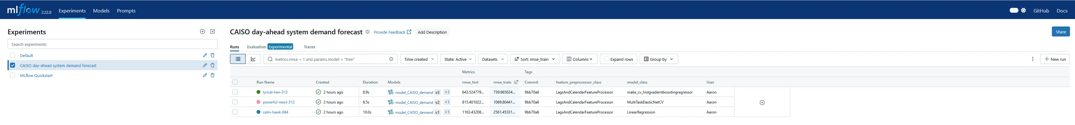
As soon as each test harness run completed, the corresponding experiment run was available in the MLflow tracking server. The UI did not refresh automatically as quickly as I expected, but manually refreshing the page took no effort. Various columns can be added to the tabular overview, including metrics and tags, so it is trivial to set up an authoritative leaderboard by experiment.

There is also a graphical view with what looks like fairly customizable plots of logged metrics, grouped by or plotted against category tags, parameters, etc. I could immediately see that some powerful dashboarding comes “out of the box” with the MLFlow tracking server and UI.

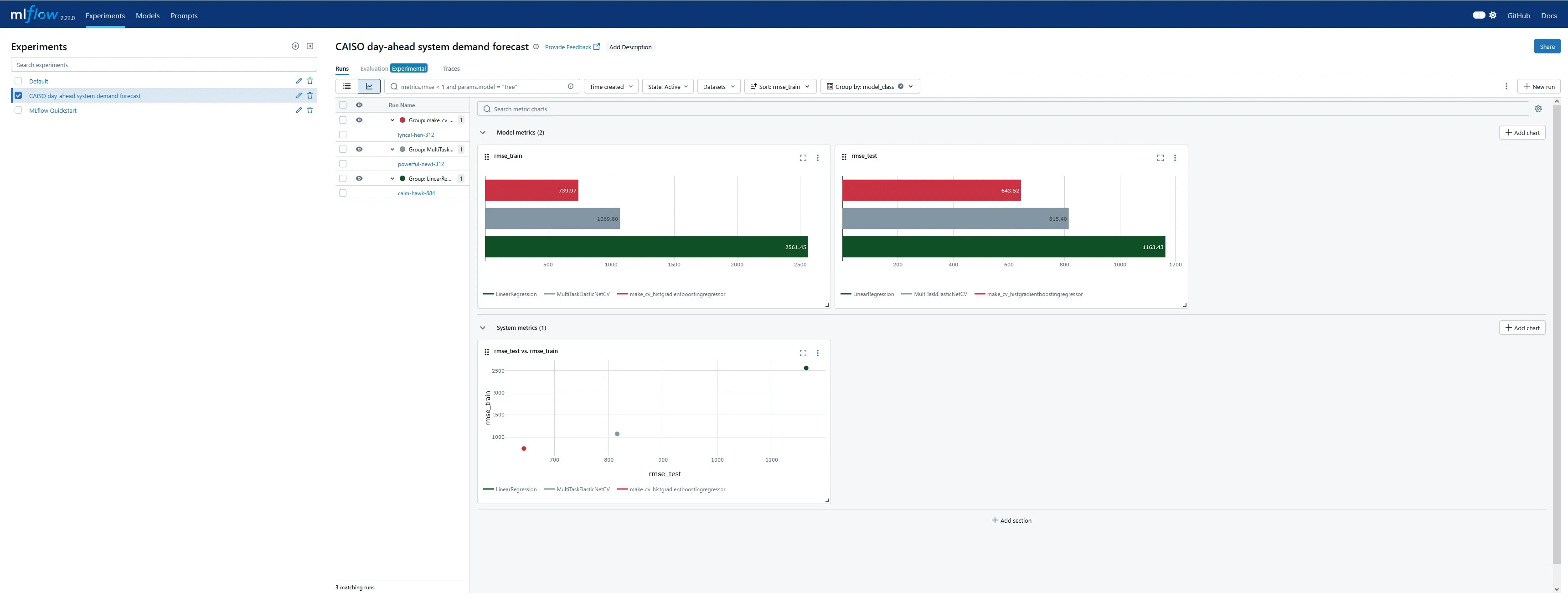
The functionality for plotting metrics against parameters on multiple axes seems deliberately intended for design of experiments (DOE), which I found very encouraging!

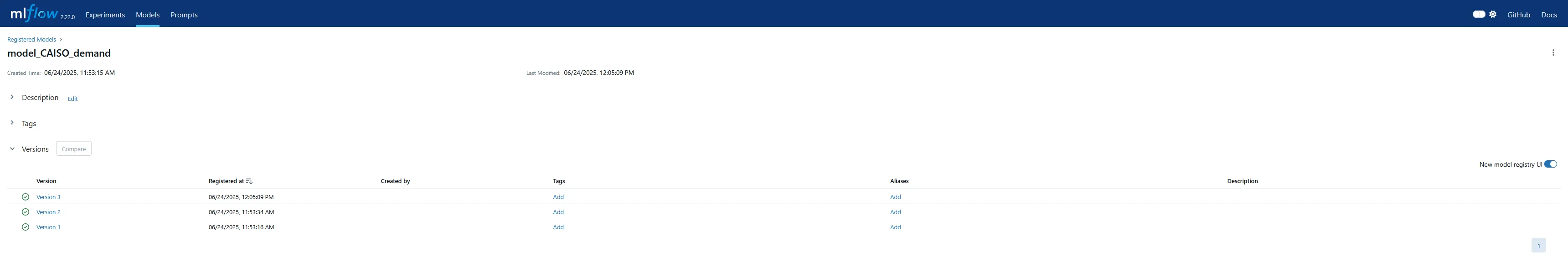
The UI has a separate tab for the model registry, which is more useful for production deployment and serving. I didn’t explore this too much in this exercise, but I was able to verify the version increments for the sub-models as each run was performed.

I also wanted to understand the distribution of forecast errors beyond just a single RMSE metric, train or test, for each experimental run. I’m not sure if MLflow can compute and plot this natively as well, but it doesn’t seem nearly as straightforward as working with scalar metrics. Instead, I set up a quick function to plot histograms of forecast errors. This is where returning the training predictions from each test harness run came in handy.

import plotly.graph_objects as go
from plotly.subplots import make_subplots

def bin_size_heuristic(sets_of_samples, nbins=24):
    """
    Quick and dirty heuristic for estimating a good histogram bin size, from
    several sets of samples, to be used for all of them.
    """
    candidates = [
        (np.quantile(s, 0.75) - np.quantile(s, 0.25)) / nbins
        for s in sets_of_samples
    ]
    return min(*candidates)

def plot_training_histograms(y, yhats_by_run, method="rmse", nbins=24):
    assert method in ["rmse", "flatten", "by_horizon"]

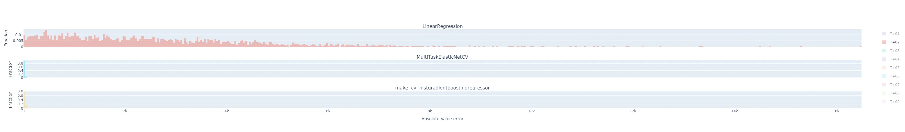
    fig = make_subplots(rows=(3 if method == "by_horizon" else 1),
                        cols=1,
                        shared_xaxes=True,
                        subplot_titles=(list(yhats_by_run.keys()) if method == "by_horizon" else None)
                        )
    i = 1  # Subplot index
    # Establish bin size from the yhats with the smallest range
    bin_size = bin_size_heuristic([y - yhat for yhat in yhats_by_run.values()])
    for run_name, yhats in yhats_by_run.items():
        if method == "rmse":
            # Take the RMSE within each day-ahead prediction, across time steps in the horizon.
            # Plot the distribution of these RMSEs across model executions.
            samples = root_mean_squared_error(y.T, yhats.T, multioutput="raw_values")
            fig = fig.add_trace(
                go.Histogram(
                    x=samples,
                    name=run_name,
                    opacity=0.33,
                    xbins=dict(
                        start=samples.min(),
                        end=samples.max(),
                        size=bin_size),
                    autobinx=False,
                    histnorm="probability"
                ),
                row=i, col=1
            )
            fig = fig.update_xaxes(title="RMSE across horizon")
        elif method == "flatten":
            # Treat every time step predicted in each day-ahead prediction run as equally important,
            # regardless of where in the horizon it is, and plot the distribution of their errors.
            samples = np.abs(y.flatten() - yhats.flatten())
            fig = fig.add_trace(
                go.Histogram(
                    x=samples,
                    name=run_name,
                    opacity=0.33,
                    xbins=dict(
                        start=samples.min(),
                        end=samples.max(),
                        size=bin_size),
                    autobinx=False,
                    histnorm="probability"
                ),
                row=i, col=1
            )
            fig = fig.update_xaxes(title="Absolute value error")
        elif method == "by_horizon":
            # Make one subplot per run, and plot the distribution of the errors grouped by horizon.
            for h in range(yhats.shape[1]):  # h-step-ahead forecast horizon
                samples = np.abs(y[:, h] - yhats[:, h])
                fig = fig.add_trace(
                    go.Histogram(
                        x=samples,
                        name=f"T+{h+1:02d}",
                        opacity=0.33,
                        legendgroup=f"T+{h+1:02d}",
                        showlegend=(i==1),
                        xbins=dict(
                            start=samples.min(),
                            end=samples.max(),
                            size=bin_size),
                        autobinx=False,
                        histnorm="probability"
                    ),
                    row=i, col=1
                )
            fig = fig.update_xaxes(title="Absolute value error", row=len(yhats_by_run), col=1)
            i += 1
    fig = fig.update_layout(barmode="overlay")
    fig = fig.update_yaxes(title="Fraction")
    fig.show()

Maybe I should have broken that plotting function apart into separate ones dedicated to each plot style, but that felt a little wasteful to me at the time. The various plot styles are as follows:

• "rmse": for each of the day-ahead (multi-horizon) forecasts in the results, compute the RMSE across the time horizons. That is, each sample in the histogram represents the RMSE of the 24 hourly predictions in that day’s day-ahead forecast. There will be $d$ samples, where $d = 2556$ is the number of days in the training dataset. All experiment runs’ histograms are superimposed so they can be compared.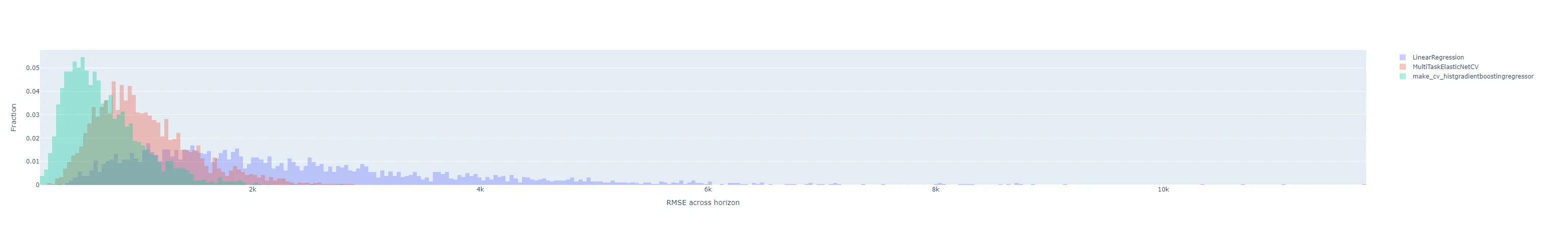

• "flatten": the absolute value of the prediction error for each horizon $h$ in a day-ahead forecast is its own sample in the histogram. There will be $24 \times d = 61344$ samples. All experiment runs’ histograms are also superimposed.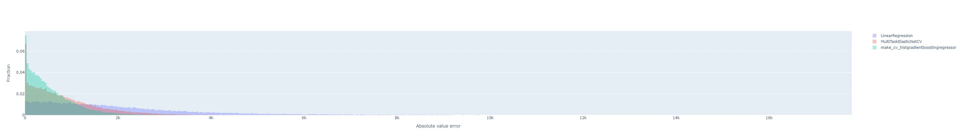

• "by_horizon": the absolute value of the prediction error, grouped by each horizon $h$, in each day-ahead forecast is its own sample in the histogram. There will be $d$ samples in each of $24$ groups. Each experiment run gets its own subplot, but the number of horizon groups is still large enough that the plot shouldn’t be interpreted with them all displayed by default. Instead, use the legend to select a single horizon to compare.

  • Let’s look at T+01 i.e. one-step-ahead forecast to illustrate. The distribution of absolute errors is widest for the naive linear regression, much tighter for the ElasticNet with hyperparameter optimization, and better yet for the Gradient Boosting regressor.
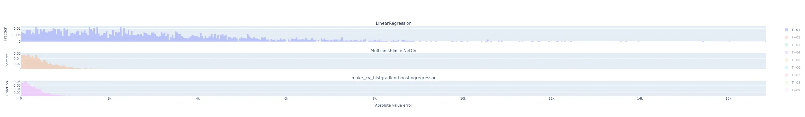
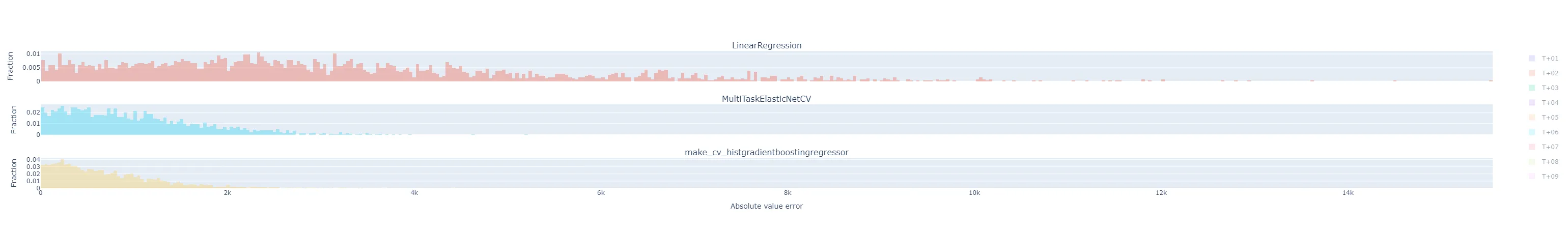
  • The T+02 errors for the ElasticNet and Gradient Boosting regressors were surprisingly low compared to other time horizons. I suspected some sort of bug or data contamination, but didn’t find anything that would explain why just this horizon - always corresponds to 4-5 PM local time - would be affected.
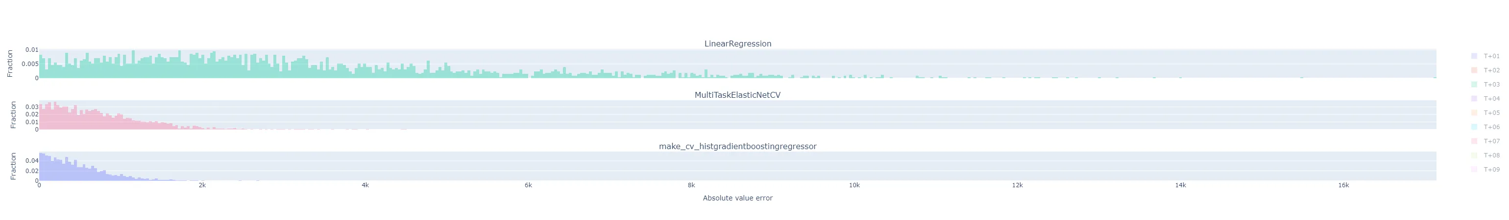
  • As I would expect, the errors generally get worse the further out the horizon is.
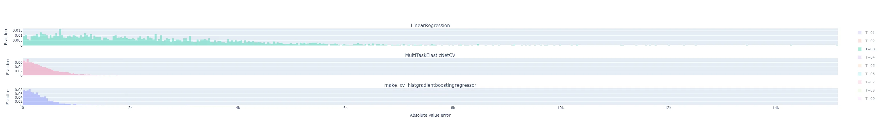
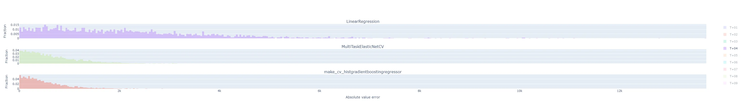
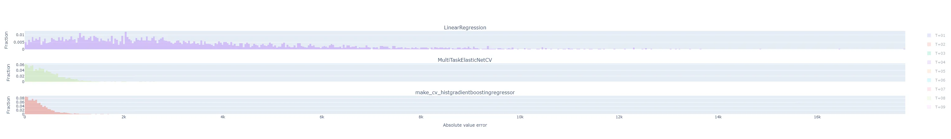
  • The following are for T+22, T+23, and T+24. As expected, they are much more difficult to predict accurately than the short-term horizons. Keep in mind that the x-axis scale changes from plot to plot.

Surprises

sklearn.base.TransformerMixin without a predict method

What happens if I try to log a feature preprocessing sub-model that doesn’t implement the predict() method? Originally, I tried using a sklearn.pipeline.Pipeline (specifically, the one in self.pipeline in the final implementation above) alone with the scikit-learn model logging flavor, mlflow.sklearn.log_model(). When the Pipeline only has scikit-learn transformers and no estimators, it has a valid transform() method but no valid predict() method. I discovered that I can perform experiment runs that log the feature engineering model, but get warnings upon logging the model:

2025/06/23 14:22:43 WARNING mlflow.sklearn: Model was missing function: predict. Not logging python_function flavor!
2025/06/23 14:22:47 WARNING mlflow.models.model: Failed to validate serving input example {
  "dataframe_split": {
    "columns": [
      "Load",
      "local_datetime",
      "inference"
    ],
    "data": [
      [
        21128.45660524064,
        "2018-01-01T00:00:00-08:00",
        0.0
      ],
      [
        20529.06680553449,
        "2018-01-01T01:00:00-08:00",
        0.0
      ],
      [
        19980.803099330882,
        "2018-01-01T02:00:00-08:00",
        0.0
      ],
      [
        19618.60789671059,
        "2018-01-01T03:00:00-08:00",
        0.0
      ],
      [
        19638.227117254075,
        "2018-01-01T04:00:00-08:00",
        0.0
      ]
    ]
  }
}. Alternatively, you can avoid passing input example and pass model signature instead when logging the model. To ensure the input example is valid prior to serving, please try calling `mlflow.models.validate_serving_input` on the model uri and serving input example. A serving input example can be generated from model input example using `mlflow.models.convert_input_example_to_serving_input` function.
Got error: Model does not have the "python_function" flavor

Still, the run succeeded and the sub-model was persisted as an MLflow model, though only under the scikit-learn flavor and not the “pyfunc” flavor. However, if I attempted to explicitly validate the training input for a serving use case, MLflow raised an error:

> mlflow.models.validate_serving_input("runs:/0d1660dfe9d24821bd35594f9cb2744a/feature_preprocessor", X_train)

---------------------------------------------------------------------------
MlflowException                           Traceback (most recent call last)
...

MlflowException: Model does not have the "python_function" flavor

So, unless a model which resembles a scikit-learn transformer gets wrapped in a class that implements predict() appropriately, at a minimum the ability to automatically validate inputs against the logged schema is forfeit. This is even if the scikit-learn flavor is successfully logged!

Timezone-aware datetime bug

I also discovered that, at the time of writing this post, MLflow doesn’t respect timezone-aware datetime columns from Pandas DataFrames when inferring a model signature or validating it. This is because internally, MLflow represents these as numpy.dtype("datetime64[ns]"), which is timezone-naive. (Contrast with datetime64[ns, UTC-08:00] for example.)

I created a Github bug ticket to report this to MLflow’s repo maintainers. For now, the workaround is that for this specific application, I should not need to track the timezone - there is only one timezone for CAISO - so I dropped the timezone prior to model fitting.

Deleting unwanted results

When working on this demo, I often wanted to delete the entire experiment and start from scratch on the tracking server if the interim results were too cluttered. This turns out to be a multi-step process. StackOverflow has a good primer on how to delete MLflow experiments permanently. In short:

• In the Models UI tab, select each model to delete. On the right-hand-side kebab menu is the Delete option.
• In the Experiments UI tab, delete an individual run by checking one or more boxes in the table view, then choosing the Delete button that appears above. Alternative, delete the entire experiment by clicking the trash can icon to the right of its name.
• Finally - and this is a necessary step - navigate to the mlruns/.trash folder in the directory where the tracking server was spun up. Permanently delete all folders in here!

Final thoughts

This investigation definitely helped me get more comfortable with MLflow and how to incorporate it into a data science project. As is often the case, testing this framework in a standalone project helped me understand the capabilities and limitations - and inspired me to ask questions! - than the quite good quickstart guides I reviewed in a past post.

I don’t think adopting MLflow into a project workflow is worth the effort for a solo data scientist. However, I am absolutely convinced of its value on a team of peer data scientists working in parallel on model development. It seems to provide quite powerful capabilities to quickly communicate the current state of model experimentation, which had been way more difficult than necessary in some of my past professional experiences! To the extent that I dipped into using the model registry to simplify versioning and deployment of models, this also appears quite powerful for relatively little setup effort. That said, I’m not sure costly this would be to scale across a large operation, and I suspect it only works if technology leadership is serious about systematizing the experimental process. The benefits of relying on MLflow’s tracking functionality only accrue if the team can, for example, consistently use a test harness like this one that eliminates the data science research process as a source of variability. I do think it’s realistic for a well-functioning data science organization to arrive at standards for these, though, making sure that they evolve over time in a way that doesn’t disrupt comparisons within an experiment (e.g. a template for all test harnesses, but within each MLflow Experiment the test harness is set in stone).

I’m curious to learn more about popular alternatives to MLflow, too. How much would a data science team benefit from adopting any systematic MLOps framework instead of ad-hoc or custom internal tooling, versus MLflow specifically? I look forward to evaluating other options in the future.