Let's explore MLflow, part 1: initial setup

Motivation

One of the challenges I’ve seen repeatedly on data science teams I’ve joined is how to get started doing MLOps in a disciplined way on a tight budget. Often there’s a homegrown procedure for machine learning model evaluation and versioning with its own custom tooling, for example, that seemed fine at first; now, the tech debt it represents is a real source of friction or even outright instability. Plenty of sophisticated vendor solutions exist, with varying degrees of how comprehensive they are - and how difficult a migration might be. Is there a simple, low-cost (ideally free for commercial use) framework that can get a team of data scientists started with “good enough”, systematic MLOps practices?

I’ve decided to explore how well MLflow works for this use case. MLflow is a free and open source MLOps platform originally developed by Databricks and now supported by the Linux Foundation. I’m mostly familiar with its experiment tracking and model registry capabilities, but nowadays it has many more features I’m interested in exploring. Importantly, it seems straightforward to self-host; I’ll evaluate this soon enough.

While I’ve used MLflow briefly in the past, I wouldn’t consider myself an expert user yet; this will be an exercise to understand how useful self-hosted MLflow alone can be for supporting good MLOps practices on a data science project. In particular, I’ll be paying attention to how easily I can:

• Reconcile artifacts like datasets, test harnesses, etc. - not just saved models - across multiple users
• Maintain a leaderboard of model experiment results across versions/users
• Abstract across wildly different model implementations with a consistent interface

The plan

Over the next several posts, I’ll walk through:

1. Installing MLflow and spinning up a local tracking server
2. Setting up a small demonstration machine learning project with one user, then eventually as if there are multiple users
3. Running experiments and evaluate ease of use

Here, I’ll focus on the the initial setup and resources to get started quickly with MLflow. Next time I’ll prepare a particular toy problem to see how straightforward it is to integrate MLflow into how I (or a small team) would work on it.

MLflow initial setup

There are two main guides provided in the online docs, a “Quickstart” and a “Tutorial”. It’s not immediately clear what the differences between them are, so I’ll evaluate both starting with the Quickstart guide.

Quickstart

Step 1: Get MLflow

Installing the package is straightforward. I created a fresh conda environment for this exercise with a pretty minimal set of packages:

conda create -n mlflow_env python=3.13 pandas scikit-learn ipykernel

Then pip install mlflow handles the rest.

Step 2: Start a local tracking server

mlflow server --host 127.0.0.1 --port 8080

If I navigate to the host/port in my browser, I see the MLflow tracking dashboard. Note that there are no experiments or runs yet (details later).

Step 3: Train a model and prepare metadata for logging

The quickstart docs provide a simple Python script for a toy example. I copied the snippets in the documentation into a Jupyter notebook for ease of use.

```python
    import mlflow
    from mlflow.models import infer_signature

    import pandas as pd
    from sklearn import datasets
    from sklearn.model_selection import train_test_split
    from sklearn.linear_model import LogisticRegression
    from sklearn.metrics import accuracy_score, precision_score, recall_score, f1_score


    # Load the Iris dataset
    X, y = datasets.load_iris(return_X_y=True)

    # Split the data into training and test sets
    X_train, X_test, y_train, y_test = train_test_split(
        X, y, test_size=0.2, random_state=42
    )

    # Define the model hyperparameters
    params = {
        "solver": "lbfgs",
        "max_iter": 1000,
        "multi_class": "auto",
        "random_state": 8888,
    }

    # Train the model
    lr = LogisticRegression(**params)
    lr.fit(X_train, y_train)

    # Predict on the test set
    y_pred = lr.predict(X_test)

    # Calculate metrics
    accuracy = accuracy_score(y_test, y_pred)
```

Note that in this example, the model training is performed first, before any calls to the MLflow tracking server are made.

So what does mlflow.models.infer_signature do? For an arbitrary object representing a model, MLflow needs to know the expected input and output formats as well as any other parameters. This schema is the model signature. Alternatively, this can be inferred by MLflow if you explicitly designate a model input example. This can be done on the fly when a model inference pass is first run, as long as the model input is of a compatible type such as pandas.DataFrame, numpy.ndarray, JSON-like structure, etc. API reference is here. Neat!

Step 4: Log the model and its metadata to MLflow

Now MLflow is invoked.

```python
    # Set our tracking server uri for logging
    mlflow.set_tracking_uri(uri="http://127.0.0.1:8080")

    # Create a new MLflow Experiment
    mlflow.set_experiment("MLflow Quickstart")

    # Start an MLflow run
    with mlflow.start_run():
        # Log the hyperparameters
        mlflow.log_params(params)

        # Log the loss metric
        mlflow.log_metric("accuracy", accuracy)

        # Set a tag that we can use to remind ourselves what this run was for
        mlflow.set_tag("Training Info", "Basic LR model for iris data")

        # Infer the model signature
        signature = infer_signature(X_train, lr.predict(X_train))

        # Log the model
        model_info = mlflow.sklearn.log_model(
            sk_model=lr,
            artifact_path="iris_model",
            signature=signature,
            input_example=X_train,
            registered_model_name="tracking-quickstart",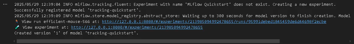
        )
```

First a new experiment is initialized, then a run within an experiment. What’s the distinction?

• An MLflow experiment represents a self-contained project or research question, which can have multiple replicates (identical) or variations. For example, this quickstart uses the famous Fisher (1936) iris dataset; the experiment here is the task to classify iris plants by species.
• An MLFLow run is a replicate or variation within an experiment. Note that the model signature used, hyperparameters, and outcome metrics are specific to a run, not to an experiment.

I’m not yet sure is this is universal, but at least in this walkthrough, I see the following:

• The run logging (log_params, log_metric) is done in the test harness. This doesn’t seem to be the only way to do it; apparently auto logging exists for commonly used, supported libraries. That said, if doing manual logging, this obviously implies that your test harness must be written with MLflow in mind, in contrast to something like TensorBoard where you just need to add a callback to start logging and visualizing results.
• mlflow.set_tag(key, value) adds a tag to the run with a key-value pair.
• While the model params, model signature, and model artifact get logged in this example, there doesn’t seem to be explicit logging of the sklearn.linear_model.LogisticRegression model class. This would allow pretty arbitrary implementations of model training/inference, as long as the model signature is provided. It’s nice this is so flexible - model training/inference could just be Python functions rather than class methods - but it also means that it might be useful to set a tag representing the model class as a standard practice. In this case, maybe it looks like mlflow.set_tag("model_class", "sklearn.linear_model.LogisticRegression"). For more complex structures such as sklearn.pipeline.Pipeline, it might suffice to log mlflow.set_tag("model_class", str(pipe)). I wonder if logging the params for a complex model object like that is as simple as mlflow.log_params(pipe.get_params(deep=True)).

For future reference, here’s a comprehensive list of all manual logging functions.

Step 5: Load the model as a pyfunc and use it for inference

```python
    # Load the model back for predictions as a generic Python Function model
    loaded_model = mlflow.pyfunc.load_model(model_info.model_uri)

    predictions = loaded_model.predict(X_test)

    iris_feature_names = datasets.load_iris().feature_names

    result = pd.DataFrame(X_test, columns=iris_feature_names)
    result["actual_class"] = y_test
    result["predicted_class"] = predictions

    result[:4]
```

The quickstart necessarily doesn’t explain why you would want to perform inference using mlflow.pyfunc instead of the native inference method of the model class, or your own custom inference function, but it’s pretty clear: this allows you to abstract across any model implementation you might be testing in the experiment! This is pretty useful if you are comparing or switching between significantly different implementations. The official docs have a very thorough explanation here. The docs claim that this works seamlessly with the currently supported production environments (e.g. AWS SageMaker, AzureML, Databricks, Kubernetes, REST API endpoints) which is extremely convenient.

I wonder how much overhead relying on mlflow.pyfunc adds.

Step 6: View the Run in the MLflow UI

Now return to the visualization dashboard.

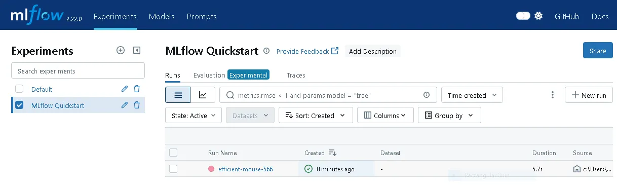
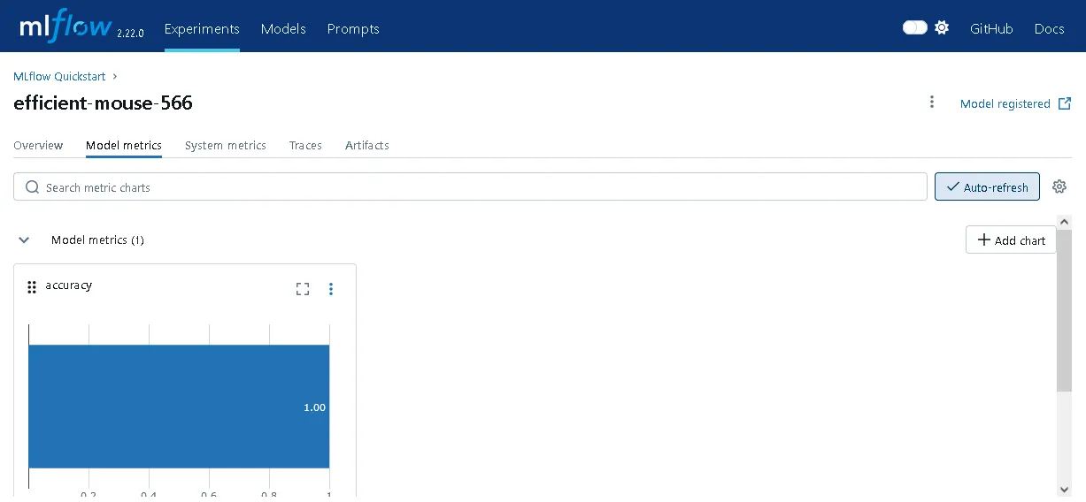
The experiment I just created is now visible, as is the training run.

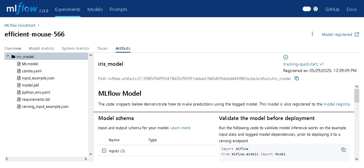
There’s even a UI tab with code snippets to support deploying the run’s artifacts to production for inference.

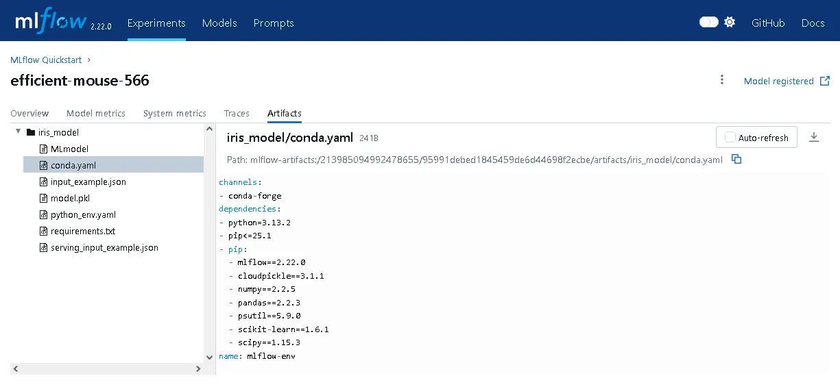
In fact, it looks like MLflow extracted the virtual environment package requirements and automatically stored them with the model artifact, e.g. a conda YAML file… this is extremely convenient! I’m really impressed.

Overall, this is exactly what I would expect from a quickstart guide! It’s a nice self-contained example, with minimal explanation of why certain steps are taken, but it’s easy enough to search in the MLflow docs for more context. Next, I’ll take a look at the tutorial guide and see how it compares.

Tutorial

Step 1: Starting an MLflow Tracking Server

This is basically identical to the quickstart’s approach.

Step 2: Using the MLflow Client API

Here I see the first main divergence from the quickstart. This tutorial now introduces the MlflowClient for interfacing with the tracking server.

from mlflow import MlflowClient
client = MlflowClient(tracking_uri="http://127.0.0.1:8080")

What is the advantage of this versus the package-level functions used in the quickstart?

This section also discusses the default experiment which can be seen in the first UI dashboard screenshot above, but wasn’t described. This is a catch-all experiment for any runs not explicitly linked to a different experiment. It seems that the best practice is to avoid using this as much as possible. There’s little downside to creating a new experiment whenever needed!

The set of all experiments, active or not, can be retrieved with mlflow.client.MlflowClient.search_experiments().

Step 3: Creating Experiments

This section has a useful discussion on when and how to organize models (runs) into experiments. The general principle is, again, that model runs should belong to the same experiment when they are substitutable (e.g. trying out different predictors for the same target; different retrained releases of the same model) or otherwise should have their performance compared “apples-to-apples”. Ironically, the example here involves forecasting demand for apples…

While the quickstart demonstrated how to tag runs, it’s also possible to tag experiments to organize them better. This is the mechanism for showing how experiments are related to each other.

I’ll just link a diagram directly from this page, as it illustrates the point very clearly:

Then the MLflow client can be used to create the experiment as well:

client.create_experiment(name=name, tags=tags)

Step 4: Searching Experiments

Now the tutorial introduces a very useful feature: filtering experiments by tag values. I completely understand why this might be excessive for the quickstart guide, but this is clearly important for getting practical use out of an MLflow deployment.

The example provided:

apples_experiment = client.search_experiments(
    filter_string="tags.`project_name` = 'grocery-forecasting'"
)

While not in the tutorial, the extended reference docs show that you can use partial matches, with % acting as a wildcard. For example, "tags.group LIKE '%x%'" will return anything with the “group” tag’s value containing “x” (case sensitive) somewhere in it.

Step 5: Create a dataset about apples

This section just covers generating a synthetic dataset to use in the next several steps.

Step 6: Logging our first runs with MLflow

The exercise of tracking a training run is very similar to what was done in the quickstart. In particular, the tutorial also uses the package-level functions that I wondered about in the Step 2 recap. Here, these are referred to as the “fluent” API. The advantage here seems to be that this simplifies integration into repeated workflows, for example by supporting context managers like with mlflow.start_run(...).

There’s an interesting side discussion at the start of this section about how the tutorial author used separate experiments while iterating through approaches for the toy problem. I understand why one would want to use separate experiments for different datasets considered, but in practice I’m not sure how useful it would be to have separate experiments for each model type. It seems to have worked for the author though, especially since the intention was to get a working nontrivial example and not to compare different models’ performance against each other per se. The main takeaway for me here is that for early stage development, it’s fine to be aggressive about eventually deleting experiments used for scratch work.

Wrapping up

As far as introductory docs go, both the quickstart and the tutorial are worth reviewing. I definitely felt that I would get immediate usefulness out of MLflow with the features covered in them alone. It’s also straightforward to imagine how multiple users could use a persistent MLflow tracking server deployment and, for example, have immediate access to a leaderboard comparing results for the same experiment.

Next, I’m going to set up my own demonstration problem and work through my own demonstration.