Building a Large Language Model from scratch, part 3

This is the third part of a series where I work through Sebastian Rauschka’s Build a Large Language Model from Scratch. The previous section covered a deep dive into the self-attention mechanism from the foundational paper “Attention is All You Need” (2017). Now, let’s evolve this into the completed GPT architecture and prepare to train and evaluate a foundational model. By foundational model, I mean an LLM that convincingly generates text to complete a provided input, but that isn’t intended to perform a specific task. That’s the aim of fine tuning, which is covered in Chapters 6 and 7 of the guide and which I’ll leave for the final post in this series.

The previous installments are here: Part 2, Part 1.

Chapter 4: Implementing a GPT model from scratch to generate text

This chapter wraps up the discussion of model architecture.Everything else beyond the core attention mechanism that goes into a GPT-like model is covered here!

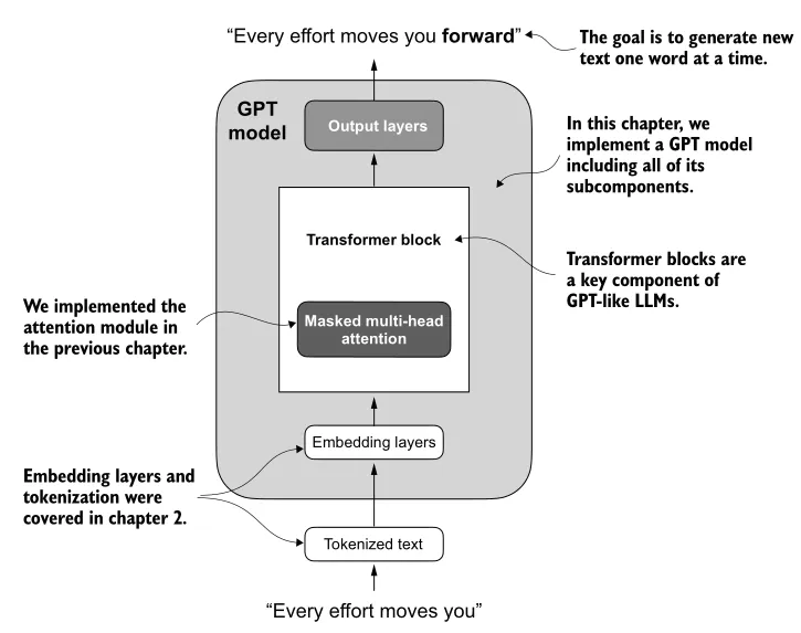
First, an overview of the simplified structure of a GPT-style LLM:

1. Tokenized text (input) →
2. Embedding layers →
3. Transformer block(s), implementing masked multi-head attention →
4. Output layers
   • First, a layer normalization (LayerNorm, to be discussed)
   • Then, a linear layer to generate logits (with output dimension being the number of tokens in the vocabulary). These logits will then be used to pick the next word.

(Source: Build a Large Language Model from Scratch, p.94)

As with the previous chapter, Rauschka starts with this high-level structure, then successively expands the level of detail down lower and lower levels of abstraction.

Normalizing activations with layer normalization

Historically, one of the core challenges for deep neural networks (DNNs) has been vanishing or exploding gradients. As a neural net architecture adds more and more layers, the gradients computed for backpropagation become numerically smaller (or arbitrarily large, depending on the operation); this leads to ineffectiveness or instability in model training respectively. In practice, this limited the possible number of stacked layers in a DNN.

Normalizing values across a layer, post-activation function, helps with this. One useful strategy, applied here, forces the outputs of a layer to have mean 0 and variance 1 through simple rescaling and shifting. The GPT architecture does this before and after the multi-head attention module in each transformer block, and also at the very end before the final output layer. Specifically, this is implemented in a custom layer that subtracts the mean and divides by the standard deviation across the feature dimension dim = -1. This is independent of batch size; contrast this with batch normalization, over dim = 0, in e.g. convolutional neural networks for machine vision. There may be advantages to adding learnable parameters to the scale and shift in this layer, too!

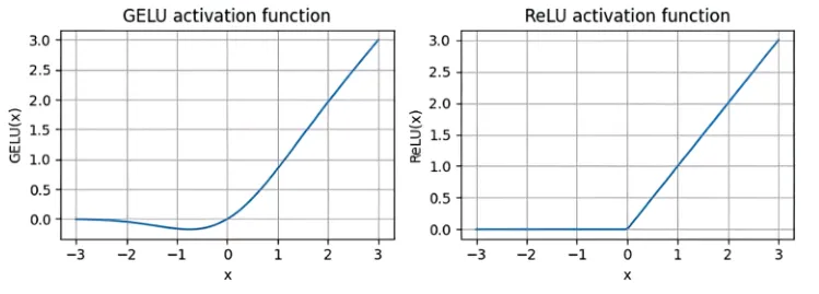
GELU activation function

The reference GPT also uses a specific activation function, the “Gaussian error linear unit”. Formally, $\text{GELU}(x) = x \cdot \Phi(x)$ where $\Phi(x)$ is the CDF of standard Gaussian distribution. This is approximated by $\text{GELU}(x) \approx 0.5 x \left( 1 + \tanh\left[ \sqrt{\frac{2}{\pi}} (x + 0.044715 x^3) \right] \right)$

Why might this be better for a GPT than a tried-and-true standard like ReLU?

• GELU is a smooth function, so its derivative exists everywhere. In contrast, ReLU is not differentiable at $x=0$. In practice, having an element of a layer output be exactly zero may be unlikely - until dropout comes into play!
• Relatedly, the derivative of GELU is nonzero everywhere, including for negative values, except for a single point near $x \approx 0.75$. For negative values, the derivative is also negative but has very small magnitude. In contrast, ReLU has a zero derivative for all negative values of $x$. This can also constrain how gradients propagate during training, as nodes that output negative values won’t contribute at all post-activation function. Historically, this was seen as a desirable property, but in practice GELU enables more efficient training of very deep networks.

(Source: Build a Large Language Model from Scratch, p.106)

The GPT architecture uses GELU as the activation function for a feed-forward neural network module that will be a component of the transformer block. This module has the following sequential structure:

1. Linear layer (tensor dimension $[b, T, e]$ → $[b, T, 4e]$)
2. GELU
3. Linear layer (tensor dimension $[b, T, 4e] → [b, T, e]$)

where $b$ is batch size, $T$ is max token length, and $e$ is the input’s embedding dimension.

The advantage of this feed-forward module seems to be that it expands the embeddings for richness of representation, then compresses them back to the original dimension. I found it interesting that this is the opposite of an autoencoder, which compresses the inputs to generate efficient embeddings that extract patterns in the data!

Shortcut connections

I’ve seen these termed residual connections or skip connections before, and I first encountered them in the 2015 paper introducing the groundbreaking image recognition model ResNet. The simple definition is that for a self-contained neural net module (say, a sequence of layers in a larger model) where the input and output have the same tensor dimension, we add the module input to its output. In practice, residual connections significantly improve trainability of very deep neural networks. Easy, right?

Rauschka frames these are yet another countermeasure to the vanishing gradients problem. That’s… not actually quite so clear-cut. How they help gradient propagation is apparently still an open question! The original ResNet paper justifies residual connections with a terse argument about learning to predict the identity function, which I attempt to summarize:

• Suppose we have an arbitrary, multi-layered neural network that we want to approximate the identity function $F(x) = x$.
• Learning the optimal weight parameters that approximate $F(x) = x$ is hard!
• Learning the optimal weight parameters that approximate the residual function, $H(x) = F(x) - x$ is easy! All the weights are zero.
• When the actual function we want to approximate resembles the identity function more than it resembles, say, $F(x) = 0$, then training its residual function will be more tractable.

To me, this last step is the most suspect. What does it mean that, in a real-world application, the function some sub-model “ought to learn” (for example, representing some useful intermediate feature of the input data) is more like the identity function than the zero function? I don’t think this is a sufficient explanation of why residual connections are so effective - and neither does the deep learning field!

An alternative explanation is that the gradient post-residual connection is the sum of the gradient of the original module (representing some complicated function with weights parameters) and the previous gradient (through the residual connection). Since this is often larger in magnitude than just the module’s gradient alone, it would inflate otherwise vanishing gradients. However, Balduzzi et al (2017) propose the mechanism of action is more subtle, addressing something they call the “shattered gradient” problem. That is, the issue here is not that the gradient of the original module is not small per se, but that it lacks informative structure. Adding the input via the residual connection reintroduces the structure from the previous stage of the model, which preserves the propagation of useful information.

The transformer block, combined

All of the above, plus the multi-head self-attention mechanism, can now be assembled into the GPT’s transformer block. Note that this module’s output has the same dimensions as the input; this makes it easy to stack multiple transformer blocks sequentially Very roughly, I interpret the structure as allowing the masked multi-head attention mechanism to learn relationships between elements in the input sequence, and the feed-forward layer to learn features of the resulting context elements. The full sequential structure of the transformer block is:

1. Layer normalization
2. Masked multi-head attention
3. Dropout
4. Residual connection (add in input)
5. Layer normalization
6. Feed Forward (Linear → GELU → Linear)
7. Dropout
8. Residual connection (add in output of step 4.)

The full GPT architecture

Finally, Rauschka can zoom out to the highest level of structure - the complete GPT model - with all of the details in place. Expanding the previously abstracted components, the GPT-2 reference model architecture looks like:

0. Tokenized text input →
1. Token embedding layer →
2. Positional embedding layer (add values into output of 1.) →
3. Dropout →
4. Transformer blocks $\times 12$ →
5. LayerNorm →
6. Linear output (word logits)

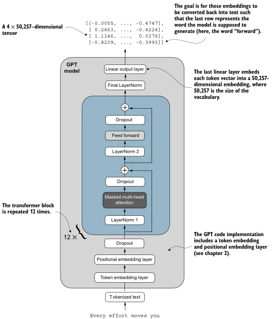(Source: Build a Large Language Model from Scratch, p.118. Contrast this with the earlier Figure 4.2; this is an example of how Rauschka iteratively refines diagrams with increasing levels of detail as he covers each topic. I found this incredibly effective for keeping track of progress!)

The GPT-2 model released by OpenAI, which this guide is based on, has been pretrained in various sizes. From here on out, the text mostly focuses on the “small”, 124 million parameter model. The model weights for all of the variants have been released to the public, but this one is large enough to yield fairly coherent output from just the foundation model, but small enough to run on a consumer laptop without a discrete GPU. My desktop’s GPU at home is sufficient for fine-tuning this model within a reasonable amount of time, and I could attempt to train it from scratch on the Project Gutenberg corpus with enough patience.

Note that this 124M parameter model appears literally to have 163M parameters. In the original architecture, weights shared the token embedding layer and the output layer shared weights in a weight tying scheme. This trades performance for memory efficiency, and in modern LLMs this is rarely done. Without weight tying, the 163M parameters at 32-bit floating point resolution require 621.83 MB. I suspect that for a given target memory footprint, there is tradeoff between parameter count (model complexity) and floating point resolution; I’d be interested to learn more about how performance changes along this frontier.

A GPT such as this one actually generates text through the following process. Each forward pass iteration yields one new token in the output, which should be appended to the context; repeat this until either the context reaches a user-specified max length, or the model emits an end-of-sequence special token.

As with previous chapters, Rauschka provides plenty of example code and worked examples of intermediate calculations. This definitely helps with building intuitions around how components of the final model work in isolation. I am very conscious of getting tripped up in aligning tensor dimensions, so these worked examples are very welcome for understanding how the shape of data changes as it flows through the network. That’s much more critical in the previous chapter than this one, though, since for transformer blocks the input and output tensor dimensions are helpfully identical!

Since this post is long enough, I’ll leave the actual demonstration of pretraining the GPT model for the next post.