Building a Large Language Model from scratch, part 1

Confession time: one of the experience gaps I’m most self-conscious about has been with large language models.

Sure, I read “Attention Is All You Need” back when it was published in 2017, and I’ve done some broad reading about transformer architecture and LLM capabilities. (The Illustrated Transformer is a really compelling visualization of how classical transformers work, by the way.) I’ve even tinkered with naively including transformer blocks in models for time-series forecasting long ago. But, to tell the truth, natural-language processing has never excited me the way other machine learning applications have. So while the LLM revolution over the past decade has profoundly impressed me - the capabilities of models from even a few years ago are the stuff of science fiction - I hadn’t caught the passion for getting deeply involved with them.

Recently it’s become clear that expertise with LLMs, or at least their foundations, is going to be indispensible for a machine learning / AI professional of any kind. Even if I’m not interested in ever building a chatbot or document summarization tool, this is not only something that I should be conversant in, but there may also be a lot of applications that I do care about where I’m leaving inspiration “on the table” if I don’t deeply understand this technology. I’ve found that the most effective way to learn something is to build it myself, even if just a prototype, and I wanted to do this with LLMs. I had been a little intimidated by the scale of the training efforts for foundation models from even a few years ago, though - is there a better entry point for a home tinkerer that won’t incur a huge cloud compute bill? I was excited, therefore, to come across Giles Thomas’ blog post series where he worked through Sebastian Rauschka’s recently published guide, Build a Large Language Model from Scratch. In short: this is exactly what I had hoped for.

What I want to get out of this

This book claims to be a hands-on exercise for how to build a tractably-sized LLM, step by step, to understand the fundamentals behind how they work. Because I already have some theoretical (if not-truly-grokked) background, mainly I want to get hands-on experience building an LLM from the ground up. 1. Understand how current LLMs do what they do, beyond just how a transformer architecture works 2. Be able to build purpose-specific LLMs for other applications 3. Apply these concepts to other domains than natural language

My plan is to take notes as I read through the text, manually retyping the example code and refactoring it in places to make sure I understand what it’s doing (and what I can and can’t change for efficiency’s sake). I’ll comment on some of the key points and my takeaways in this blog, but I won’t rehash each chapter’s content comprehensively. For that, just pick up the book itself!

Chapter 1: Understanding large language models

This chapter is an introduction to LLMs and why one would want to use them. Even without any technical background in LLMs or NLP in general - and the book does not assume any, beyond some intermediate Python programming experience - this is a good overview at a pretty high level.

One aspect I particularly like about Raushka’s book is that even early on, it lays out the general strategy of, well, how to build an LLM from scratch and fills it out across multiple levels of abstraction. For example, this first chapter already has a section introducing the transformer architecture, which sketches it out at an intermediate level of detail. Diagrams representing data flow or model architectures are presented multiple times, starting with the first chapter, at increasing resolution. There’s a particular diagram - Figure 1.9 - that appears multiple times at various milestones in the text, and it serves as both a visual table of contents (for the reader) and a process flow diagram (for the practitioner). I found this very appealing.

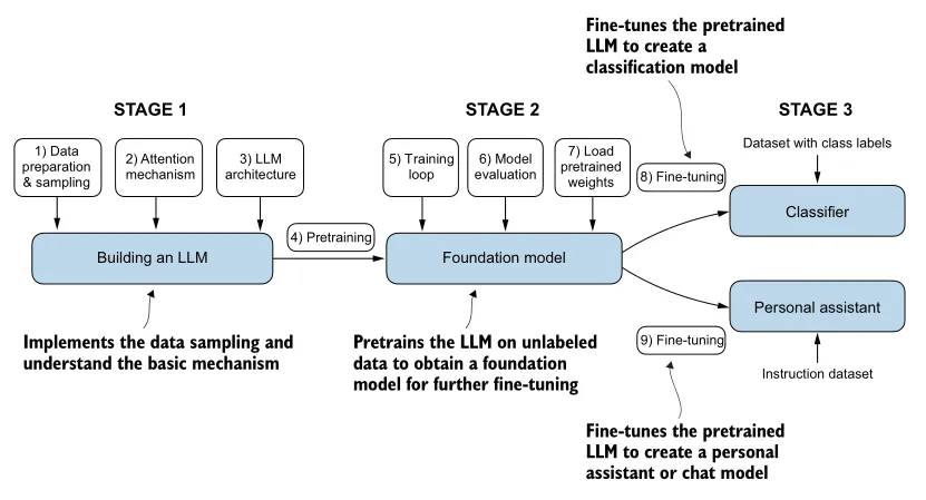(Source: Build a Large Language Model from Scratch, p.14)

This figure is itself a low-resolution version of the roadmap. Each of the elements in the three stages shows up in an expanded version of this diagram when its topic is covered in the relevant chapter. In my option, this is really effective in making sure the reader doesn’t get lost despite the serious complexity! For example, the Chapter 3 text works through several toy versions of the attention mechanism, each one a little more accurate than the last, in order to gently introduce the core ideas and build upon them. It’s valuable to be reminded of where this is situated in the grand scheme of things, and the payoff it works towards.

Chapter 2: Working with text data

This chapter sets the stage for understanding natural language processing (NLP) problems in general. Note that this applies to other models for NLP applications, not just LLMs; some of these techniques have been around for decades. Without getting into excessive historical background, the section is a concise but good overview of what it means to take natural language data and convert it into a form that machine learning models can use. There are two key aspects of this:

1. Tokenization: how to represent words (or parts of words) as discrete numerical values.
2. Embeddings: how to represent those as points in a continuous space.

Tokenization

Roughly put, the motivation behind tokenization is that machine learning algorithms need to operate directly on numerical, not character, data. The text data fed into an LLM can be thought of as a sequence of words, punctuation, and other characters. Tokenization is the step of converting this into a sequence of IDs, or tokens, representing the relevant building blocks of text.

A naive way to do this is to build a vocabulary of all the possible words and punctuation marks a model should be capable of handling, and build a 1-1 map between those and unique IDs. Note that for English texts, this is on the order of 10,000s of unique tokens, which is large but not a huge memory burden. It is useful to include other special tokens in the vocabulary, for example to represent an unknown word, or the end of the sequence. Relatedly, one of the drawbacks of the naive approach is that it’s not very robust to words in the input text which are not found in the tokenizer vocabulary, including proper names.

A preferred way to tokenize text is byte pair encoding. This is a more sophisticated approach used by GPT models, and efficient libraries exist for this such as tiktoken. Roughly, when a full word in the input text is not in the vocabulary, the tokenizer breaks it down into subword units (morphemes) or even individual letters. (The byte pair encoder’s vocabulary is built during training by iteratively combining letters into subwords and subwords into words, depending on how frequently the combination of sub-units shows up in the corpus. The full details are outside the scope of Build a Large Language Model from Scratch.) This is why I referred to “building blocks of text” above; they’re not necessarily literal words!

Embeddings

The more interesting piece, in my opinion, is how these tokens are transformed by embeddings. The core idea is that we want a way of representing words in a continuous numerical space rather than as discrete tokens, because that would allow us to do arithmetic on words… and construct functions of words… and take gradients of those functions of words… and that allows us to write machine learning algorithms that operate on words! We can achieve this if we can represent, somehow, each word as a coordinate in space - an embedding space - and build a mechanism that maps each word’s token ID to a coordinate.

(Side note: I found it interesting that for the kinds of LLMs described in this guide, we don’t need a mechanism that translates arbitrary embedding coordinates to, say, the closest word in the embedding vocabulary. To skip ahead quite a bit, that’s because the output of a GPT can simply be a neural net linear layer with one node per word in the vocabulary, and the value of each is the logit of the probability that it’s word is the next one in the sequence! No inverse embedding required!)

Clearly, there are many ways to assign unique coordinates in an $N$-dimensional space to words in a vocabulary; which scheme is optimal? It depends on the application, which suggests that the scheme should be trained… say, with a machine learning model! Historically this was often done by dedicated, separate deep learning models such as Word2Vec, but nowadays LLMs commonly produce their own embeddings during training.

A valuable embedding scheme will represent relationships between words that reflect their meanings. The classic example is a 2D embedding where, in the embedding space, $king + (woman - man) = queen$. The dimension of the embedding space can be arbitrary, though it should probably be much smaller than the expected vocabulary size, and is itself a hyperparameter for learning an optimal mapping.

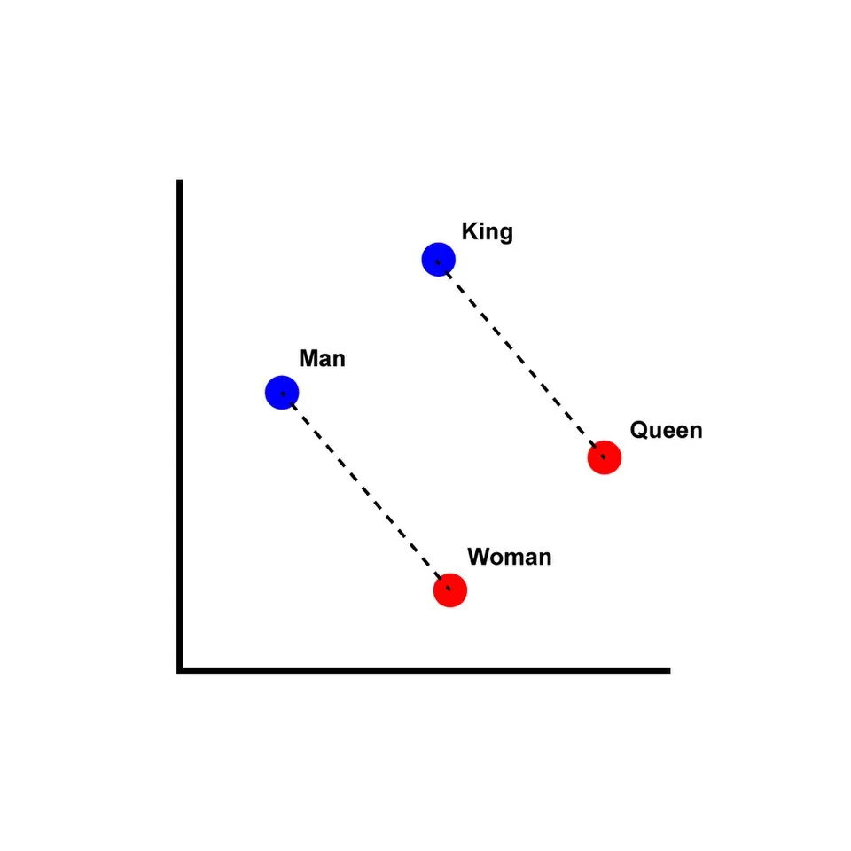(Source: Wikimedia Commons)

One final comment on this topic: embeddings can be constructed for other data such as audio or video content, not just words. In fact, learning embeddings for entire documents (representing, say, the topic of each document in a way that encodes their relationships to each other) is a key enabler of retrieval-augmented generation.

Data sampling with a sliding window

With the previous two mechanisms implemented, we can convert chunks of text input into sequences of vectors (i.e. coordinates in the embedding space representing tokens). The remaining major topic in this chapter is how to slice up and fetch these sequences for training a GPT-style LLM.

A specific variant of LLM, generative pre-training (GPT) models iteratively predict the next token in a sequence. Since the remainder of the book focuses on GPTs, the input-target pairs for model training are $(\text{the tokens prior to } t, t)$ for each token $t$ in each training document. In principle, it would be good to start with the first token in a document and incrementally grow the input, so that the training records are cumulative over the length of the document. In practice, the input (“context”) should be implemented as a “sliding window”:

• “Context size” is how many previous tokens to use to predict next one. This is necessary because a fixed input sequence length must be specified when constructing the model architecture.
• “Stride” is how many tokens to skip from one example to the next in a training batch. Stride = 1 yields a new example for each token, whereas stride = context size yields examples that are totally disjoint. This is necessary because too much overlap, i.e. a small stride, generally leads to overfitting.
• Batch size is a speed/memory tradeoff and is a tunable hyperparameter.

The strategy that Rauschka takes in his example Python code is to subclass PyTorch’s Dataset and DataLoader classes, implementing in them the tokenization and data sampling approaches but handling the token embedding in the LLM architecture. Token IDs are converted to embeddings by a specialized embedding layer within the LLM. This is functionally equivalent to one-hot encoding followed by fully connected linear layer, trainable via backpropagation.

LLMs also benefit from encoding word positions in the input context. By themselves, token embeddings don’t capture position in a sequence. LLM task performance has been found to improve, however, when feeding in an additional feature representing position in a sequence. Critically, this feature isn’t concatenated to the embedding for each input token - it’s added to the embedded vector. (I’m still not completely sure why it couldn’t be concatenated instead to increase the input vector size, to be fair. Is it for memory efficiency?) For this reason, this feature is called positional embedding, and the final embedding vector is therefore the token embedding plus the positional embedding. Rauschka discusses two approaches to constructing the positional embedding: absolute and relative.

• Absolute positional embedding: each position in sequence has a unique value, e.g. token 0, token 1, …
• Relative positional embedding: the value is relative to number of tokens prior to the target. One advantage of this is that it generalizes across sequences of different lengths.

In practice, one or the other may be better depending on application. The original transformer model used deterministic, absolute positional embeddings. These were a sinusoidal function of token position, and to be honest, were initially very confusing for me when I first encountered it. The Illustrated Transformer has a more accessible treatment of it that helped me quite a bit. More recently, OpenAI’s GPT models optimize the weights applied to the positional encodings themselves during training.

While all of the text’s Python code is available in the book’s repo, I decided to write my own Jupyter notebook instead, using the book example code as a a starting place. The sample code is extensive and written for ease of understanding first. For instance, mechanisms taught in the text will be implemented with for-loops instead of more efficient but less legible constructs. Only later on does Rauschka revisit these with improved implementations that illustrate techniques for better efficiency. I found this teaching approach very effective for removing any unnecessary complexity at each stage. In a guidebook like this, there’s no need to be prematurely concise!

In my next blog post, I’ll move on to Chapter 3. In many ways this is the most important section of the book, and it’s certainly the most complex: building the transformer architecture from first principles.